install.packages("shiny")
library(shiny)5 Shiny apps
Shiny applications, in short shiny apps, are applications created in r with a shiny user interface. We have seen for the first time the shiny user interface in Chapter 3 when we created parameterized reports.
shiny apps are extremely useful when the goal is to engage with the audience or readership or supervisors in an interactive and dynamic manner. This application type is powerful because it builds on the programming language r and integrates user design features.1 2
Here are examples of shiny apps from my work and others.3
1 - Predicted as observed created by Dr. Julian Kohnke. Read explanation paper by Witte, Stanciu, and Zenker (2022).
2 - Quantum social sciences created by myself. Read explanation preprint by Witte and Stanciu (2023).
3 - Elements of cross-cultural research created by Maksim Rudnev.
Generally, I feel that the beginner’s guide on the official shiny website is more than enough. In this section, we will cover only the basics and address some of the tricky and subtle knowledge about writing code for shiny apps. There are not many, but the few that are can become frustrating.
To make things a bit more interesting, we will transform the parameterized report build in Chapter 3 into a shiny app while adding a few additional interactive features to it.
The official shiny beginner’s guide is simple, useful, and full of fun and interactive examples. Navigate to this guide here.
The set-up
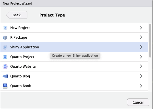
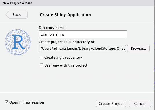
Figure 5.1 should by now be a familiar routine: We create an R project that has a default working app. Once you’ve created the project, you will note only one file: app.R (next to the .Rproj extension, of course).
The .R file format is an r script file format. Meaning, that you can write r code, save it and even run it without having to transfer the code to the console. Remember that in RMarkdown and quarto documents, we worked with r code chunks. Well, the .R script files are much like a gianormous code chunk.
Remember the dataset Stanciu et al. (2017) introduced in Chapter 1? We will use it in creating our very own shiny app.
Note that r script files can hold only basic code meaning that features from RMarkdown and quarto are not available. If you’d like to integrate HTML or other languages, that is possible, but requires appropriate integration which we do not cover here.
If everything went well, we should have the shiny package already installed from Chapter 1. But, if you haven’t done so yet, or are unsure about it, now is a good time to install this package.
R script files
.R script files can be very useful not only for shiny apps but also for websites or books. Writing code in such file format can keep the work environment neat and tidy. Also, you might want to use script files when you know in advance that you have repetitive code (e.g., functions) that you use across several of your projects.
One example where I personally apply this work strategy is when writing my own functions (see Chapter 2). Instead of writing a function each time I would need it, I include all functions I create into an .R script file which I then copy-paste to all my projects. Other strategies are possible, for example, install all packages in a separate script file or divide the work flow in programming into several steps - data import, data cleaning, data manipulation, data analysis, and data ready to report.
When working with code stored in separate script files we need to call these into the main document, for instance, in an RMarkdown, quarto or shiny app.
This is easily done with the function source("{yourrscript here}"). Make sure that the path dependency is correct and that the script is wrapped around " ".
When we work with data saved in an R format such as .Rds and .Rdata, we can call this dataframe using the function load("{your .Rdata dataframe here}"). Remember the path dependencies and the " "!
Before we start working on the shiny app let us save the data (Stanciu et al. 2017) into an .Rdata format. This makes it somewhat easier to import the dataframe in the shiny app code, as it is already in an r format.
Building on the code written in Chapter 3, we save to an .Rdata file format.
# imports data in SPSS .sav format
dfex<-haven::read_sav("data/sample.sav")

# saves R object dfex into an .Rdata format
# which we load into the shiny app shortly
save(dfex,file="data/sample.Rdata")
In Chapter 2 we wrote a basic function to add a constant to all numeric columns to a data frame. We can copy this function into an .R script so that we have access to it in writing our first shiny app.
Create a new .R script file by navigating to File/ New File/ R Script. It will open an empty untitled script file. Copy the function as is into this script file.
func1<-function(df,n){

  tmp <- Filter(is.numeric, df) # we first filter the dataframe for numeric columns

  tmp + n # we then add the constant to all the numeric columns
}r scripts
Note that if you write custom scripts and store them inside r script files, you’d need to make sure that the required packages are called inside that script file. Use the install.packages() or library() commands as described in Chapter 2.
Shiny apps structure
What makes shiny apps powerful and at the same time a bit tricky to program is the structure. Shiny apps have a user interface (UI) that is wrapped around code that runs in the background on a server. When programming a shiny app therefore we need to program both the design (UI) and the code that runs on the server (server).
The UI part makes a shiny app attractive to the audience and, if programmed right, can engage the audience in an interactive and dynamic manner. Programming the UI part requires a bit of orientation toward the audience for which the app is designed. What are the minimum skills required to operate the app? What theoretical and practical expertise is expected for the audience to intuitively navigate the app? Read more on user interface in general on the Wikipedia page.
The server part makes a shiny app, well, work. Here is where code is written to import, clean, manipulate and analyse data, metadata and all sorts of other things. One way that I find helpful to think of the server part is to see it as the old-school R coding on my local machine. When you use r for data analysis, for example, you use this programming language in the console which then you run resulting in some form of output. Well, this means technically that you interact with your computational machine (CPU, for example) through the r programming language. This very principle applies also for writing code for the server for shiny apps.
This distinction is less intuitive when we run the shiny app on the local machine. But, this distinction between UI and server becomes crucial when we deploy the app on online repositories, as we will see shortly. By deploying the app code structured into UI and server, we tell the respective servers how to read our code.
So, long story short, both the UI and server segments of a shiny app code has its own pre-defined role and it is crucial for the well functioning of the app that this structure is maintained. Otherwise the app breaks.
Code for UI
This will not be a comprehensive code at all. But, it should offer sufficient hands-on tips on how to start building your UI for your first shiny app.
One thing to keep on the back of your mind is that in the UI part we need to refer to objects from the server part. If we do not call objects from the server in the UI part properly, the app might still work but the audience will not have access to it.
Make sure that you always use commas and close the brackets appropriately. Otherwise, the design might not look as intended or the entire code might break even.
My recommendation is to take some time to decide what do you want to include in the app and what do you need for your audience. For example, do you want the audience to view plots or tables, and if yes, do you want these to be interactive? If that is the case, what code do you need to write on the server part and what is the final r object that you’d want to be displayed for the audience via the UI?
So, for me at least, writing a shiny app is a bit of a forth and back between the UI and server code.
5.0.1 Layout
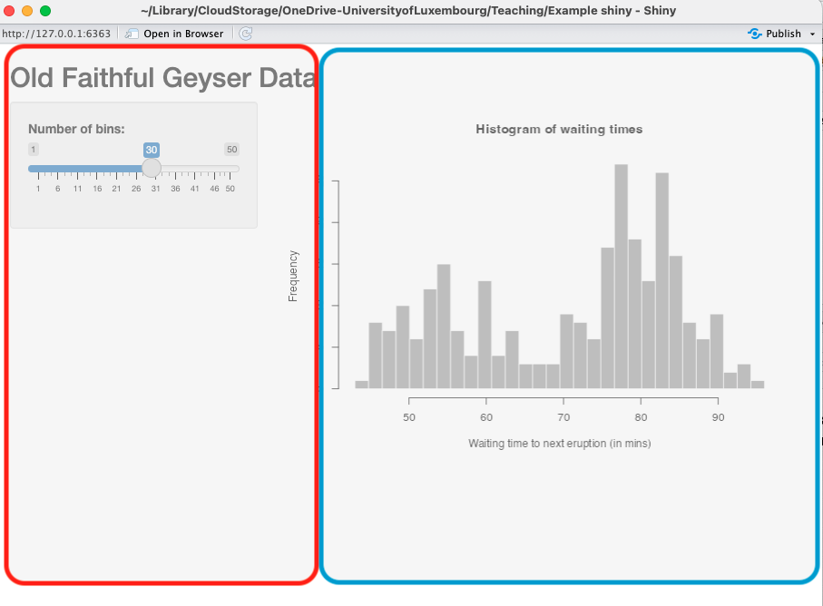
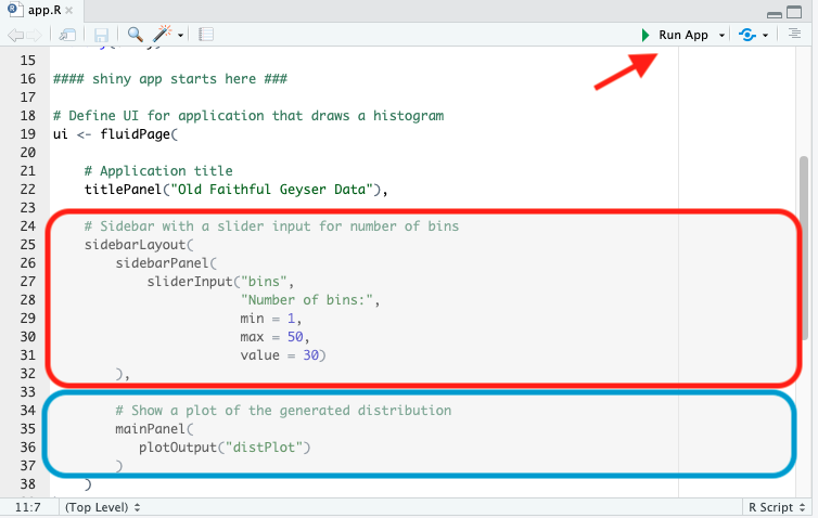
sidebarLayout(): Inside this function we define the content that will be displayed on the side of the app window. See red panel of Figure 5.2 (a) and the corresponding red panel in Figure 5.2 (b). One can also add elements to the layout of this panel. For example try out the code below and see what happens.
# copy and paste this code line as the first argument inside the
# sidebarLayout() function followed by a comma
# I cannot stress this enough: Commas are super super important
# so do not forget them

position = "right"sidebarPanel(): This is wrapped inside the sidebarLayout() because it is just one element of several that can be placed on the sidebarLayout of the app.
The attributes defined here are fed into the code on the server, so make sure you chose the appropriate user input type.
mainPanel(): This contains the output, be it plain text, live text, tables or figures. If in the sidebarPanel() you define the user input attributes, in the mainPanel() you simply call the objects computed on the server and programm how exactly will they be displayed. See in blue Figure 5.2 (a) and the corresponding code in blue inside the UI Figure 5.2 (b).
5.0.2 Input types
Inside the sidebarPanel() we can define the kind of user input we expect our audience to play with. That is – remember parameterized reports from Chapter 3 – what are the parameters that users can interact with. There are a couple of input types, for example, slider input on a continuous pre-defined numeric range, select from a pre-defined list, check if TRUE or FALSE, and a numeric only text field.
sliderInput(): This is given as an example in the default shiny app that comes pre-set when creating a shiny app project. It is a slider input type. Observable are five attributes:
Label of the input
"bins"which is a reference label for the codeLabel of the input displayed to users (
"Number of bins:"). Note that this is different than input label above and serves only the function of informing the user. The input label above serves the function of cross-reference in code writing.minandmaxdefine the minimum and maximum of the numeric range of the slider.valuedefines the default value of the slider which is displayed every time the app is called.
selectInput(): This is a select from a pre-defined list input type. In the basic form, it requires three attributes:
Label of input for cross-referencing in the code.
Label of input for display for the app users.
Values of the pre-defined list. Note that these should be places inside a list, which has this basic structure:
c("{NAME 1 TO BE DISPLAYED}" = "{value 1 for code cross-referencing}",
"{NAME 2 TO BE DISPLAYED}" = "{value 2 for code cross-referencing}"...)
It may look like this (code from Witte and Stanciu (2023)).
selectInput("hov",
          "Choice: ",
        c("all",
          "Openness to change" = "och",
          "Conservation" = "con",
          "Self Transcendence" = "str",
          "Self Enhancement" = "sen")
)#closes selectInputcheckboxInput(): This is a yes/ no logical input type. Ideally, you always define at least three atributes:
Label of input for cross-referencing in the code.
Label of input for display for the app users.
valueis true (value = T) or false (value = F).
It may look like this (code from Witte and Stanciu (2023)).
checkboxInput("p1.ess","Distribution", value = F)numericInput(): This an input type that allows the user to type in numeric values within a pre-defined range with a pre-defined increment value. One can define the following:
Label of input for cross-referencing in the code.
Label of input for display for the app users.
valueis the default value show every time the app is opened.minandmaxdefine the range of possible values within which the user can choose to enter from. Note that this range is not visible to the user but it is a by-design-limitation. An error is shown or simply the input is not validated if the user enters a value outside this pre-defined range.stepdefines the increment value. It can be a full integral number or anything inbetween.
It may look like this (code from Witte and Stanciu (2023)).
 numericInput("n",
                                  label = "Sample size",
                                  value = 20,
                                  min = 20,
                                  max = 1000,
                                  step = 1)
5.0.3 Conditional panels
There might be situations where you’d want to create a conditional user interface. This means that the UI experience can, at some pre-defined parts, be conditional on user input. For instance, for the app Quantum Social Science, I created a UI dependent on type of analysis: choice. There are three choices the user can select: Simulations, Survey data or Experimental data (which is still under construction). Depending on the user choice at this stage, the user has different options to choose from - either interact with simulated data or with secondary data.
It may look like (code from Witte and Stanciu (2023)).
  conditionalPanel(
            condition= "input.type=='Simulations'",
... # the code continues here with input valuesconditionalPanel(): Wrapped inside one can code the UI conditional on an input defined at a previous stage. Let us pay a closer look at the example above:
condition = "input.type=='Simulations'":
condition =introduces the condition that needs to hold for the contents of the rest of conditionalPanel to be activated."input.type=='Simulations'"is the condition itself which is to be read as follows: if the input of input object “type” is identical to “Simulations”, then the subsequent contents are activated. See Figure 5.3.
5.0.4 Tabset
There can be situations where it is helpful to organize output into separate panels – similar logic to having several tabs open on your web browser.
The app Predicted as observed created by Julian Kohne for the paper Witte, Stanciu, and Zenker (2022) nicely uses this feature.
In the mainPanel() the “Abstract” of the paper, followed by “Check assumptions”, the calculation of the “Similarity Index” and display of the “Similarity Interval”, and, finally, “Recommendations” are organized neatly into tabs. The user can navigate these tabs knowing the kind of content to expect.
tabsetPanel(): defines the overall structure within which multiple panels can be placed.
tabPanel(): defines the content be placed inside a tab. This is coded inside tabsetPabel()!
It may look something like this.
tabsetPabel(
  tabPanel1("label 1 for display to user", {content 1 here}),
  tabPanel2("label 2 for display to user", {content 2 here})
)
Code for server
The code for the server is a custom function, a gianormous custom function! Like any custom functions (see Chapter 2), there is a structure to it, namely function(){}.
The server function takes two arguments, namely input and output.
input signals what comes from the UI interface. That is, what the user of the app is inputing via the UI.
output signals what goes from the server to the UI. That is, what the user views as a result of interacting with the app.
5.0.5 Reactive objects
The simplest way to think of reactive objects is to see them as plain old-school R code wrapped inside an object that the server needs to compute. It is reactive, because the server has to first compute the reactive object before performing any tasks that call on such an object.
In r code written for computation on the local machine it would be called simply an r object.
On the server, however, code is computed only when needed which makes objects created on the server reactive to code that requires them. They react if you poke them. Otherwise, they sleep.
This is one of those ultra small details that took me days to figure out. When you create a reactive object, remember to always call it as such. It is an r object all right, but it looks like a function: reactiveobject().
A reactive object, like all objects coded for the server, need to be wrapped in a specific function, otherwise the server will not recognize it as such.
Code for the server – whether it is reactive, input or output objects – needs to be written inside ({YOUR SERVER CODE HERE}). It is a specific code chunk for the server. Its logic is similar to the code chunk introduced in Chapter 3 – it is a field recognized by the server as code to be computed.
Once a reactive object was coded following the code structure introduce in Tip 5.7, the reactive object itself can be called inside other code on the server following the structure presented in Tip 5.6.
5.0.6 Input objects
Technically speaking, input objects are reactive objects. But, I discuss them separately because these feed user input to the code.
This can be recognized and done by adding the prefix input$ when calling user input.
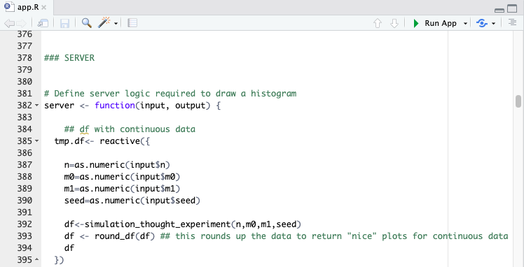
In the code example from Witte, Stanciu, and Zenker (2022) (see Figure 5.4 (a)), a reactive object tmp.df is coded at lines 385 – 395.
This reactive object happens to be using user input information as indicated at lines 387 – 390.
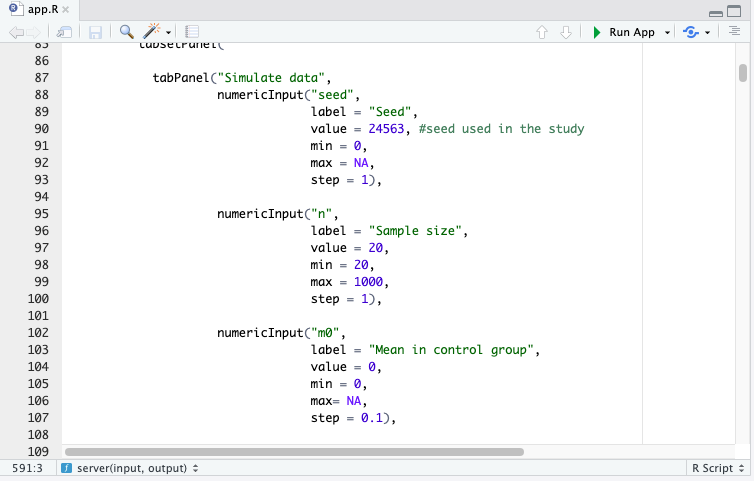
To illustrate the correspondence between UI and the server, see in Figure 5.4 (b) the user defined object n at lines 95 – 100 and the user defined object m0 at lines 102 – 107.
5.0.7 Output objects
Output objects are the output that we want to be displayed on the user interface. This means that we have to call it as such and indicate the position where we want it displayed.
Ideally, we have already coded the display position and display characteristics in the UI code.
On the server, we need to indicate the object corresponding to the UI code accordingly. When we feed user input to the server code we write the prefix input${USER INPUT}. Well, when we want an object displyed on the user interface we write the prefix output${corresponding label in the UI code}.
Note the dollar sign $!
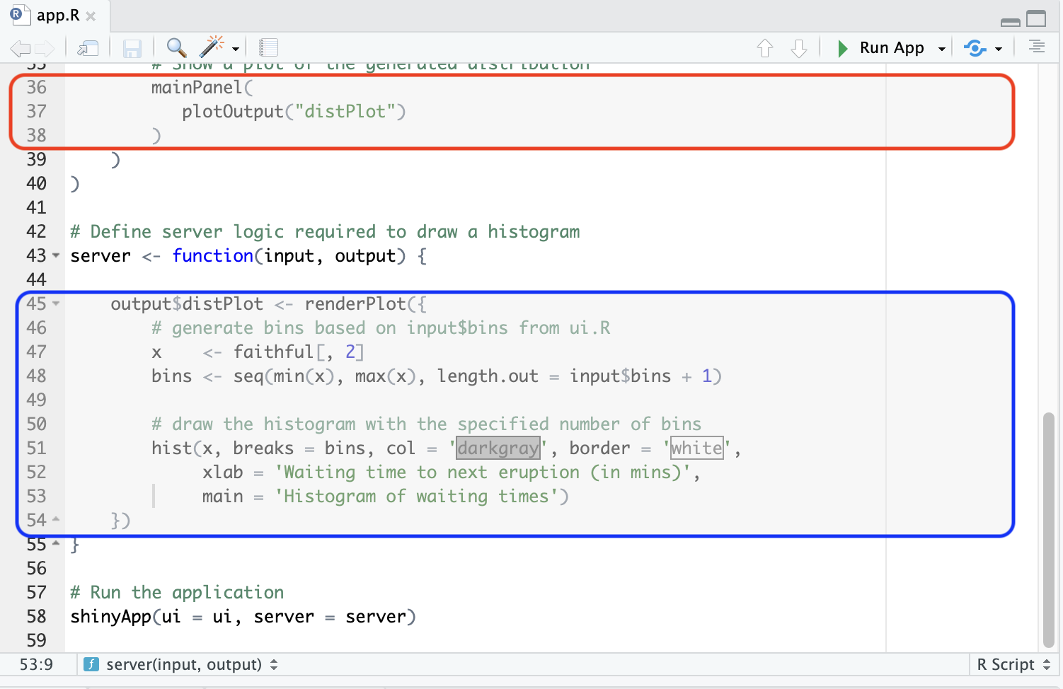
In Figure 5.5 (a), we see at lines 36 – 38 (red field) the UI code for object distPlot to be displayed. At lines, 45 – 54 (blue field), we see the server code for this object. Finally, in Figure 5.5 (b) (blue field), we see the output plot displayed for user experience.
When writing output objects, these need to be wrapped inside designated code chunks – for plots or tables or text. See this official cheat sheet.
Run the app locally
Running the app locally is as simple as pressing the button Run App on the bar – see for instance Figure 5.2 (b).
Note however that this is in fact calling a function written inside the app.R script.
This function is shinyApp(ui = ui,server = server). The shinyApp() function takes two arguments ui and server which we define separately, as indicated above.
A new window will open. You might note two things in the console:
The console is busy with the app, as indicated by the STOP symbol.
The text in the console Listening on {an IP address}.
These two things indicate that the app is running and that the console cannot be used for other purposes. It also means that the app is automatically updated if you are to modify the code, UI or server. It also means that your local machine acts as the server in this case.
The moment you close the app, the console becomes available once more.
Deployment
To deploy the app, we would need a dedicated server and, of course, an access account on that server. One efficient and smooth way to deploy a shiny app online is to use the dedicated server shinyapps.io. It is a free service maintained by the same community behind RStudio – posit.co.
To start with, open an account on shinyapps.io. Once you have an account, we can turn back to our app that we’ve coded in RStudio.
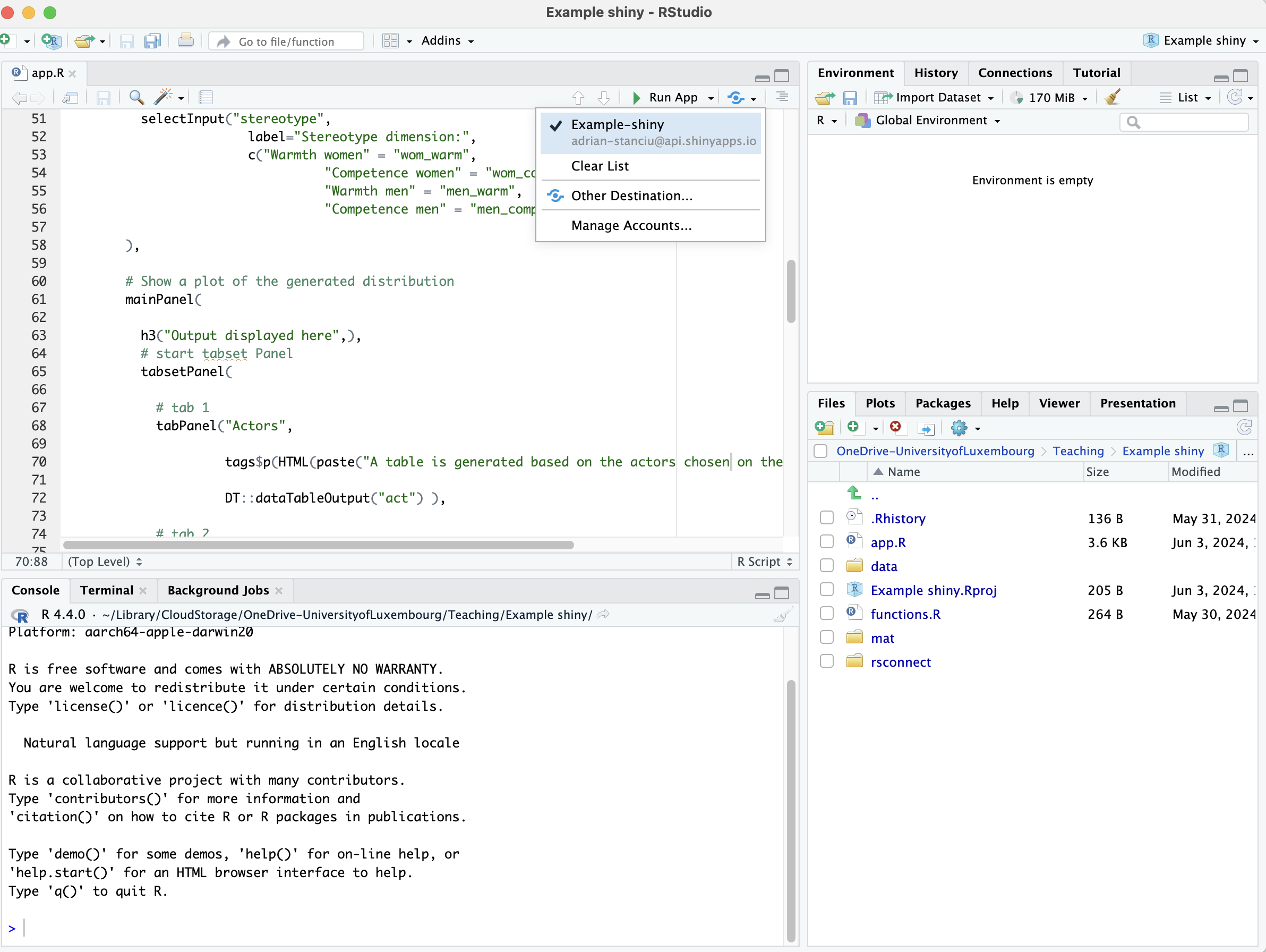
Next to the button Run App there is another button called Publish the application or document. Click on it and follow the steps as indicated. Note that in Figure 5.6, the app has already been deployed so there is a connection with the external server made. If you publish an app for the first time, you will only see the option Publish Website.... Select from the options shinyapps.io and follow the instructions. In a matter of a few secods your app will be online!4
Not all files are needed for the final app to function. When you deploy the app, select those files from your local repository that the app actually needs to function. By doing this, you make sure that the server is not filled with junk. After all, your free shinyapps.io account has limited space.
The illustrative example is deployed online here. See also sub-section below.
(Optional) Push to GitHub
One further thing we might want to do is to push the script files to GitHub as discussed in Chapter 4.
Try doing that yourself. I pushed my script files on a public GitHub repository that can be accessed here5.
Progress illustrative example
Below is the entire code for the illustrative example that was transformed from a parameterized report into a shiny app.
You can try to replicate it by yourself and compare it with mine. Or copy paste it directly into a app.R script and run it. The choice is yours.
### calls r script files
source("functions.R")

### loads data
load("data/sample.Rdata")

### imports libraries
library(shiny)

r <- getOption("repos")
r["CRAN"] <-"https://cloud.r-project.org/"
options(repos=r)

# install.packages("pacman")

# pacman::p_load(tidyverse,readxl,haven,sjlabelled,kable,kableExtra)

#### shiny app starts here ###

# Define UI for application that draws a histogram
ui <- fluidPage(

    # Application title
    titlePanel("Illustrative example"),

    # Sidebar with a slider input for number of bins
    sidebarLayout(position = "left",

        sidebarPanel(

          # actor input
          selectInput("actor",
                      label="Choose an actor:",
                      c("Keanu Reeves",
                        "Alec Baldwin",
                        "Arnold Schwarzenegger",
                        "Timothee Chalamet",
                        "Anamaria Marinca"),
                      multiple = TRUE),

          # stereotype input
          selectInput("stereotype",
                        label="Stereotype dimension:",
                        c("Warmth women" = "wom_warm",
                                  "Competence women" = "wom_comp",
                                  "Warmth men" = "men_warm",
                                  "Competence men" = "men_comp"))

        ),

        # Show a plot of the generated distribution
        mainPanel(

          h3("Output displayed here",),
          # start tabset Panel
          tabsetPanel(

            # tab 1
            tabPanel("Actors",

                     tags$p(HTML(paste("A table is generated based on the actors chosen on the side panel..", sep = "")) ),

                     DT::dataTableOutput("act") ),

            # tab 2
            tabPanel("Stereotypes",

                     tags$p(HTML(paste("A plote is generated based on the variable chosen on the side panel..", sep = "")) ),

                     plotOutput("st") )

          ) # close tabset Panel
        )
    )
)

# Define server logic required to draw a histogram
server <- function(input, output) {

  ####### -- imports and prepares data from here

  # reactive object
  # data from Stanciu et al. 2017

  tempdf <- reactive({

    choice=input$stereotype

    dfex %>%
      sjlabelled::remove_all_labels() %>%
      pivot_longer(contains("warm") | contains("comp")) %>%
      filter(name %in% choice)

  })

  # reactive object
  # meta data movies
  movietmp<- reactive({
    dfmv<-readxl::read_excel("mat/movies.xlsx",1) %>%
      filter(Actor %in% input$actor)

  })

    #### -- generates output objects from here

  # generate ggplot
  plottmp<- reactive({

    ## ggplot code
    (input$plot_type == "ggplot2")

    ggplot(tempdf(), aes(x=factor(gen),y=value)) +
      labs(title=paste0("Evaluation based on ", input$stereotype),
           x="Gender",
           y=paste0("Stereotype of ", input$stereotype)) +
      geom_boxplot() +
      theme_light()
  })

  ##### -- code for output from here

  # render plot for user
  output$st <- renderPlot({

    plottmp()
  })

  output$act <- DT::renderDataTable({

    movietmp()
  })
}

# Run the application
shinyApp(ui = ui, server = server)
Note however that you’d still need to create all the external scripts and r data files.
Advanced resources
If you really really like shiny apps and want to master them, then this book by Hadley Wickham contains everything one needs to know. Other online resources are available and offer varying levels of complexity.
pythonprogramming language is likewise supported but won’t be covered in this short book. See the official website for more.↩︎One can integrate
shiny appfeatures inquartodocuments as described here.↩︎Some of these apps might take a bit of time until they load because they might be “asleep”. A shiny app is asleep when there is no activity for a pre-determined time thus the server cleans up working memory by putting inactive apps to sleep.↩︎
Connecting to the server and deploying the app might take some time. Once the app has been successfully deployed, it will open automatically in your default web browser.↩︎
Note that you need to be logged-in to your
GitHubaccount to see the script files↩︎

